
The following description tends to assume a pattern classification problem, since that is where the BP network has its greatest strength. However, you can use backpropagation for many other problems as well, including compression, prediction and digital signal processing.
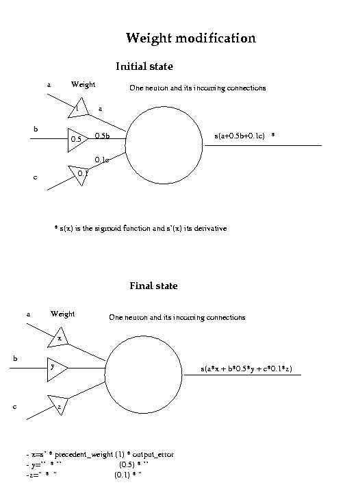
When you present your network with data and find that the output is not as desired, what will you do? A good answer would be: we will modify some connection weights. Since the network weights are initially random, it is likely that the initial output value will be very far from the desired output.
This begs the question: which connection weights will you modify, and by
how much? To put it another way, how do you know which connection is
responsible for the greatest contribution to the error in the output?
Clearly, we must use an algorithm which efficiently modifys the different
connection weights to minimise the errors at the output. This is a common
problem in engineering; it is known as optimisation.
The famous LMS algorithm was developed to solve a similar problem, however the neural
network is a more generic system and requires a more complex algorithm to
adjust the many network parameters.
One algorithm which has hugely contributed to neural network fame is the back-propagation algorithm, which consists of the following steps:
A neural network is useless if it only sees one example of correct
output. It cannot infer the characteristics of the input data which you are
looking for from only one example; rather, many examples are required.
This is analogous to a child learning the difference between (say) different
types of animals - the child will need to see several examples of each to be
able to classify an arbitrary animal.
If they are to successfully classify birds (as distinct from fish, reptiles etc) they will need to see examples
of sparrows, ducks, pelicans and others so that he or she can work out the
common characteristics which distinguish a bird from other animals (such as
feathers, beaks and so forth). It is also unlikely that a child would
remember these differences after seeing them only once - many repetitions
may be required until the information `sinks in'.
It is the same with neural networks. The best training procudure is to
compile a wide range of examples (for more complex problems, more examples
are required) which exhibit all the different characteristics you are
interested in. It is important to select examples which do not have major
dominant features which are of no interest to you, but are common to your
input data anyway.
One famous example is of the US Army `Artificial Intelligence' tank classifier.
It was shown examples of Soviet tanks from many different distances and angles on a bright sunny day, and examples US
tanks on a cloudy day. Needless to say it was great at classifying weather,
but not so good at picking out enemy tanks.
If possible, prior to training, add some noise or other randomness to your example (such as a random scaling factor). This helps to account for noise and natural variability in real data, and tends to produce a more reliable network.
If you are using a standard unscaled sigmoid node transfer function,
please note that the desired output must never be set to 0 or 1! The reason
is simple: Whatever the inputs, the outputs of the nodes in the hidden layer
are restricted to between 0 and 1 (these values are the asymptotes of the
function. To approach these values would require enormous weights and/or
input values, and most importantly, they cannot be exceeded.
By contrast, setting a desired output of (say) 0.9 allows the network to approach and
ultimately reach this value from either side, or indeed to overshoot.
It cannot be overemphasised: a neural network is only as good as the training data! Poor training data inevitably leads to an unreliable and unpredictable network.
Having selected an example, we then present it to the network and generate an output.
In our neural network problem, we take all output numbers from the neural network output layer and calculate the difference between this value and the desired value, for example in the following example we have in the output 0.1 and 0.9 and the desired outputs 0.2 and 0.85 so, the error found will be 0.1 and -0.05. Since a single overall measure of error is required (so we can say whether the overall output is `acceptable' or not), the mean square value is used (simply, the sum of the squares of the errors divided by the number of outputs). In this case, the MSE is 0.00625.
| Resulting output | Desired output | MSE |
|---|---|---|
| 0.1 | 0.2 | (0.2 - 0.1)^2 + (0.9 - 0.85)^2 = 0.00625 |
| 0.9 | 0.85 |
To minimise this parameter, we should consider the error at the output
(for a given input and desired output) as a function of the network weights.
Consider the output layer.
With a given input to the layer and desired output from the layer,
the actual output is simply a complicated function of
the network weights. It is clearly a function of a very large number of
variables, since if we have N nodes in the current layer and M nodes in the
previous layer, there are a total of MN weights connecting the two layers.
The error as a function of the network weights can be thought of as an MN
dimensional surface (the `error surface').
Therefore, we wish to get to a state of minimum error (the lowest point on the surface)
from the point where we currently are, located elsewhere on that surface. The simplest
approach is to calculate the gradient vector (that is, a set of gradients in
each dimension) of the surface at the point we are currently at, and make a
small step in the opposite direction. This takes us lower on the surface,
and closer to the desired minimum. Fortunately, if we use a simple transfer
function for the nodes (such as the sigmoid) the gradient may be calculated
simply, in fact it becomes a function of the sigmoid itself. This is useful
since it reduces the number of calculations - the output values of the
network may be re-cycled when evaluating the gradient.
The new values for the network weights are calculated by multiplying the negative gradient with a step size parameter (called the learning rate parameter) and adding the resultant vector to the vector of network weights attached to the current layer. This change does not take place, however, until after the middle-layer weights are updated as well, since this would corrupt the weight-update procedure for the middle layer.
Clearly, the error at the output will be affected by the weights at the middle layer, too. However, the relationship is more complicated. A new error function is derived, but this time the output weights are treated as constants, the inputs are constant, and the desired output is constant. Now, the actual output is a function of the weights attached to the middle layer only (and there are LM of those, for L input nodes and M middle-layer nodes). Fortunately, it is still a relatively simple expression. The middle weights are updated using the same procudure as for the output layer, and the output layer weights are updated as well. This is a complete training cycle for one piece of training data.
It should be noted that the input layer is really only a buffer to hold the input vector. Therefore, it has no weights which need to be modified.
This process is analagous to the biological process of learning - the strength of individual connections between the neurons increases or decreases depending on their `importance'.
Since we have only moved a small step towards the desired state of a minimised error, the above procudure must be repeated until the MSE drops below a specified value. When this happens, the network is performing satisfactorily, and this training session for this particular example has been completed.
Once this occurs, randomly select another example, and repeat the procedure. Continue until you have used all of your examples many times (`many' may be anywhere between twenty or less and ten thousand or more, depending on the particular application, complexity of data and other parameters).
Finally, the network should be ready for testing. While it is possible to test it with the data you have used for training, this isn't really telling you very much. Instead, get some real data which the network has never seen and present it at the input. Hopefully it should correctly classify, compress, or otherwise process (however you trained it!) the data in a satisfactory way.
A consequence of the backpropagation algorithm is that there are
situations where it can get `stuck'. Think of it as a marble dropped onto a
steep road full of potholes.
The potholes are `local minima' - they can trap the algorithm and prevent it from descending further.
In the event that this happens, you can resize the network (add extra hidden-layer nodes or even
remove some) or try a different starting point (i.e. randomise the network
again).
Some enhancements to the BP algorithm have been developed to get
around this - for example one approach addes a momentum term, which
essentially makes the marble heavier - so it can escape from small potholes.
Other approaches may use alternatives to the Mean Squared Error as a measure
of how well the network is performing.
| Previous | Contents | Next |